Mining, processing, and visualizing Twitter data using rtweet, TidyText, and tidyverse

Data, Data, Everywhere

We live in a day and age where data is being generated at a pace that is faster than ever! Much of this data is also unstructured, untidy, and now also dominated by text format. Lately, I have been exploring the utility of the tidytext package to process such messy natural language data and draw insights. Thanks to the open source #rstats community, processing untidy unstructured data is easier than ever!

In this short example, we will grab the Twitter data using the rtweet package, process it using tidytext and tidyverse, and visualize it using ggplot and leaflet.

🔍 Searching for Tweets

First, let us load all the packages we will need. We will use the rtweet package to query the tweets, tidytext, and tidyverse to clean and mine the text data, and ggplot and leaflet for visualization. rtweet is an R client for accessing Twitter’s REST and stream APIs. We will use ggthemes package to upgrade the theming of our plots.

library(rtweet)
library(tidytext)
library(tidyverse)
library(leaflet)
library(ggthemes)

As an example, let’s scrape tweets that use the hashtag ‘#omicron’ in them. We can do this using the search_tweet() function from the rtweet package.

tweets <- search_tweets(q = "#omicron", n = 18000,
                                      lang = "en",
                                      include_rts = FALSE)

🧹 Cleaning the data

Let’s peek into the raw tweet data

tail(tweets$text)

## [1] "And finally Quebec opened the schedule for 25-35 yo. It was about time... Still 3 weeks to wait though. I will be Pfizer'd³ at the beginning of February. <U+0001F489><U+0001F489><U+0001F489> #vaccine #vaccin #vaccination #pfizer #3rddose #omicron https://t.co/6eC5rOdD7n"
## [2] "Great <U+0001F9F5>on #Omicron - what we know to date* in simple and accessible language.\n\n*as of January 12, 2022 (some in pre-print stage), so things may change https://t.co/m9nPRgMU2s"                                                                          
## [3] "Trying to stay up to date on the latest news regarding #COVID19? Epidemiologist and guest writer for the @nytimes, @ShamanJeffrey, sheds light on when to expect #omicron to peak as well as how these projections are made. Read more here: https://t.co/GACw22mEPV."
## [4] "2785 New COVID+ve cases reported in Jaipur today!\n\n#NewsCapital #Coronavirus #coronaviruspandemic #coronavirusoutbreak #COVID19jaipur #COVID #Corona #COVID19rajasthan #India #Covid19upate #Omicron #omicronindia #Jaipur #Rajasthan https://t.co/twvb0JAu1y"      
## [5] "If the virus is on the way to become endemic, hospitalisations are less than 20% and Asymptomatic patients account for approximately 84% of those testing positive, then why are we treating this wave as being at par to Wave 1 or 2? #GenuineKoschan #Omicron"      
## [6] "Amazing! \n“We have already started manufacturing for the commercial scale of #Omicron vaccine. We anticipate to be ready for market supply by March 2022, subject to regulatory approval.”\nhttps://t.co/1YuvQmvaxp"

At the first glance, it is clear that there is quite a bit of data cleaning required. For example, you may want to remove URLs from scraped tweets. You may even want to get rid of emoticons, punctuation, etc. while at it. As an example, let us remove the URLs from the tweets and look at the data.

tweets<- tweets %>%
  mutate(stripped_text = gsub("http.*","",text))

tail(tweets$stripped_text)

## [1] "And finally Quebec opened the schedule for 25-35 yo. It was about time... Still 3 weeks to wait though. I will be Pfizer'd³ at the beginning of February. <U+0001F489><U+0001F489><U+0001F489> #vaccine #vaccin #vaccination #pfizer #3rddose #omicron "        
## [2] "Great <U+0001F9F5>on #Omicron - what we know to date* in simple and accessible language.\n\n*as of January 12, 2022 (some in pre-print stage), so things may change "                                                                                           
## [3] "Trying to stay up to date on the latest news regarding #COVID19? Epidemiologist and guest writer for the @nytimes, @ShamanJeffrey, sheds light on when to expect #omicron to peak as well as how these projections are made. Read more here: "                  
## [4] "2785 New COVID+ve cases reported in Jaipur today!\n\n#NewsCapital #Coronavirus #coronaviruspandemic #coronavirusoutbreak #COVID19jaipur #COVID #Corona #COVID19rajasthan #India #Covid19upate #Omicron #omicronindia #Jaipur #Rajasthan "                       
## [5] "If the virus is on the way to become endemic, hospitalisations are less than 20% and Asymptomatic patients account for approximately 84% of those testing positive, then why are we treating this wave as being at par to Wave 1 or 2? #GenuineKoschan #Omicron"
## [6] "Amazing! \n“We have already started manufacturing for the commercial scale of #Omicron vaccine. We anticipate to be ready for market supply by March 2022, subject to regulatory approval.”\n"

Now that the URLs are gone, the text starts to look a bit cleaner. However, you might not want to do all the cleaning manually. Thankfully, the tidytext package comes with the unnest_tokens() function that works like magic and cleans up all the text. It converts the text to lowercase, gets rid of punctuation marks, and adds the unique tweet id for each occurrence of the unique word. Let us use it over our URL-stripped text data.

tweets_clean <- tweets %>%
  dplyr::select(stripped_text) %>%
  unnest_tokens(word, stripped_text)

🙊 What is the chatter about?

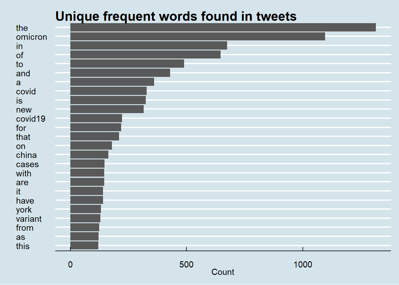
Let us grab and plot the 25 most frequent words from our data.

tweets_clean %>%
  count(word, sort = TRUE) %>%
  top_n(25) %>%
  mutate(word = reorder(word, n)) %>%
  ggplot(aes(x = word, y = n)) +
  geom_col() +
  xlab(NULL) +
  coord_flip() +
      labs(x = "",
      y = "Count",
      title = "Unique frequent words found in tweets")+ggthemes::theme_economist()

🧹 More cleaning

Spot any potential problems with this plot? Looks like we need to clean up the data even more. We need to filter all the ‘stop words’(e.g. in, and, a, of, etc.). Again, thanks to the inbuilt stop_words data included with the tidytext package, we can swiftly remove all the filler words from the text. Let’s test it out with our data.

Before filtering out the stop words our tweets_clean data contains 484151 observations.

tweets_clean <- tweets_clean %>%
  anti_join(stop_words, by = "word")

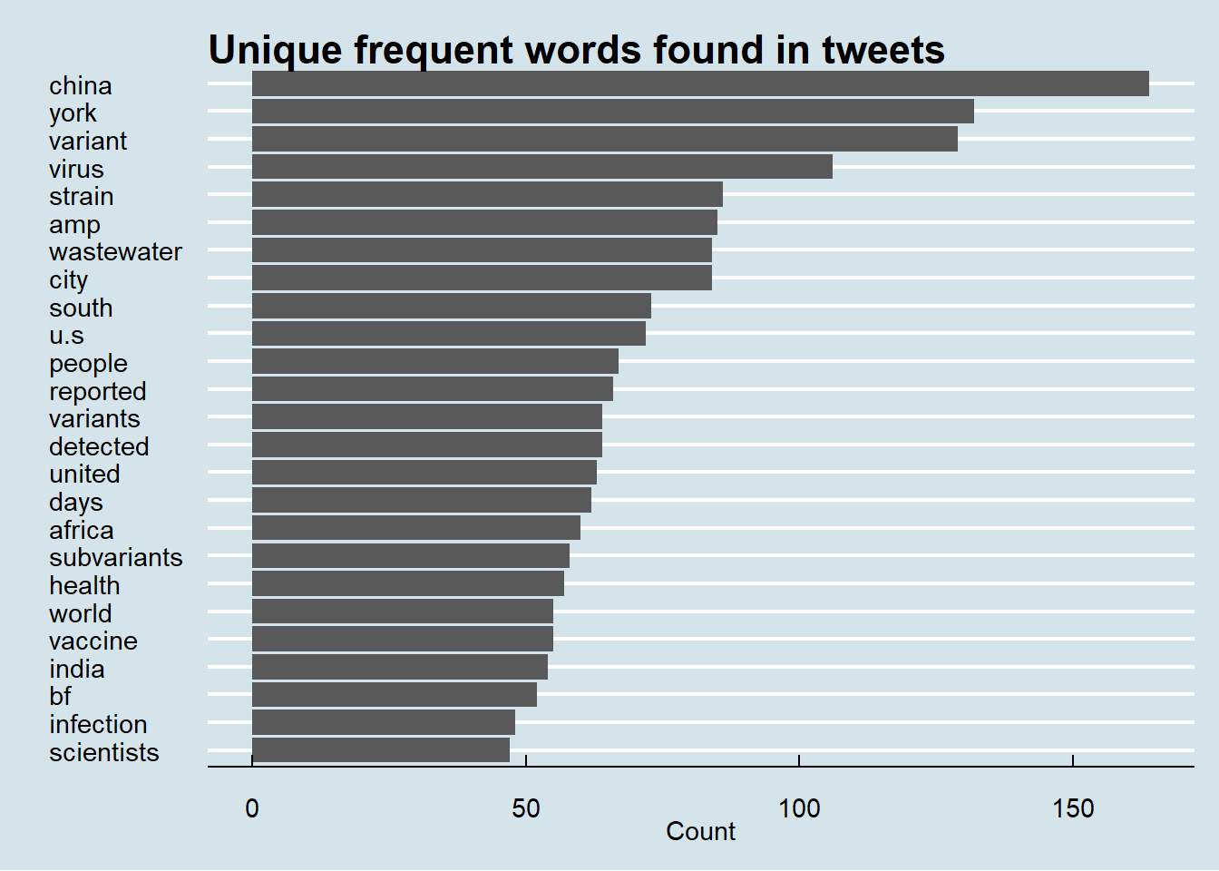
After filtering out stop words our data has 285218 observations. We can also filter out the numbers/integers and the terms related to our query (such as delta, covid19, etc.) that might mask our actual results.

tweets_clean <- tweets_clean %>%
  dplyr::mutate(word = gsub('[[:digit:]]+', '_', word)) %>% 
     dplyr::filter(!str_detect(word, "omicron|covid19|covid|delta|coronavirus|_")) 

Let us now recreate our previous plot with this clean data.

tweets_clean %>%
  count(word, sort = TRUE) %>%
  top_n(25) %>%
  mutate(word = reorder(word, n)) %>%
  ggplot(aes(x = word, y = n)) +
  geom_col() +
  xlab(NULL) +
  coord_flip() +
      labs(x = "",
      y = "Count",
      title = "Unique frequent words found in tweets")+ggthemes::theme_economist()

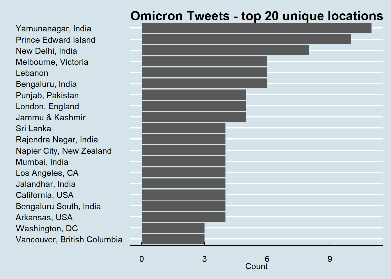
🗾 Mapping the tweets

To find out where these tweets come from, we first need to add the latitude and longitude information for each tweet. This can be done using the lat_lng() function from the rtweet package.

tweets_with_latlons <- rtweet::lat_lng(tweets)

tweets_with_latlons %>%
  count(place_full_name, sort = TRUE) %>%
  mutate(location = reorder(place_full_name,n)) %>%
  na.omit() %>%
  top_n(20) %>%
  ggplot(aes(x = location,y = n)) +
  geom_col() +
  coord_flip() +
  labs(x = "",
       y = "Count",
       title = "Omicron Tweets - top 20 unique locations ")+ggthemes::theme_economist()

Let us create a spatial map of these tweets.

leaflet::leaflet() %>%
  leaflet::addProviderTiles(leaflet::providers$OpenStreetMap.Mapnik) %>%
  leaflet::addCircles(data = tweets_with_latlons, 
             color = "blue")

Now, let us make this map interactive and display in the pop-up a set of hashtags that are being tweeted from each location. And there we go!

tweets_with_latlons %>% leaflet::leaflet() %>%
  leaflet::addProviderTiles(leaflet::providers$OpenStreetMap.Mapnik) %>%
  leaflet::addMarkers(popup = ~as.character(hashtags),
                      label = ~as.character(hashtags))